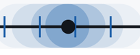
The decision is binary. The measurement shouldn't be.

Hamel Husain has taught thousands of engineers how to evaluate LLM applications, and the evals FAQ he writes with Shreya Shankar has become a standard reference for the field. This week he answered one of its most frequent questions on X (his post): why use binary pass/fail labels instead of 1-5 Likert ratings? His full FAQ answer is worth reading first. We agree with most of it, and the part we would add is small but useful.

What Hamel gets right

Uncalibrated 1-5 scales are noisy. The FAQ says the gap between a 3 and a 4 is subjective and inconsistent across annotators, that people drift to the middle, and that you need larger samples to see a real difference. Every measurement person has seen this. A five-point scale with no anchors and no model behind it is less reliable than a well-defined yes/no check, and retiring it is good advice.

Binary labels also make error analysis faster. They force you to write down what "bad" means, which is the hardest and most valuable part of early evals work, and they keep annotators from hiding in the middle of a vague scale.

The decision really is yes or no. You ship the prompt or you don't. The guardrail trips or it doesn't. Any eval that never ends in a clear decision is not doing its job.

His best idea is the one most people skip. For tracking gradual progress, the FAQ recommends several binary sub-checks, such as "4 out of 5 expected facts," rather than a 1-5 accuracy score. That example is where his view and ours meet.

Two jobs, not one choice

The question "binary or continuous?" quietly assumes we must pick one. We need both. Faithfulness, helpfulness and harm severity come in degrees, so the measurement should be continuous. The release gate is yes or no, so the decision should be binary. Likert was the wrong way to measure, but that does not make continuous measurement the problem.

His "4 out of 5 expected facts" already shows this. It is an ordered count from 0 to 5, which is a graded scale built from binary checks. The useful question is not binary versus continuous. It is whether the scale is calibrated, and where the pass/fail line sits on it.

Signal detection theory separated these two jobs 70 years ago

Signal detection theory treats every yes/no judgment as two parts: a continuous evidence value, and a criterion (call it x_c) that turns the evidence into a verdict (Peterson, Birdsall, & Fox, 1954; Green & Swets, 1966). Moving x_c trades hits against false alarms. Sensitivity, d', is a separate quantity that tells you how well the evidence tells good outputs from bad ones (Macmillan & Creelman, 2005).

A binary label squeezes both of those into one bit. If judge A fails more outputs than judge B, the label can't tell you whether A is sharper or just stricter. Once you keep the continuous score, the two questions come apart: one is about how good your measurement is, and the other is about where you put the line.

Industry measures first, then decides

Manufacturing settled this a long time ago. To accept or reject a part, you measure the characteristic, state the uncertainty of that measurement, and compare the result to a specification limit. When consumer risk matters, you add a guard band (JCGM 106:2012). Six Sigma puts lower and upper spec limits on a continuous characteristic, and capability indices like Cpk can only be calculated from variables data, not from pass/fail counts (Montgomery, 2012).

Qualifying the gauge follows the same logic. A variables gauge study splits error into repeatability (one rater, repeated) and reproducibility (between raters). An attribute agreement study only reports how often people agreed, and it needs far more trials to reach comparable confidence (AIAG, 2010). The factories that ship millions of parts measure on a continuous scale and make the decision at the end.

Dichotomizing throws data away

Cutting a continuous variable into two groups has a known cost. A median split of a normally distributed variable multiplies its correlation with anything else by about 0.80, so the variance it explains drops to about two thirds. Cohen (1983) described this as being like discarding roughly a third of your data. Later reviews kept reaching the same verdict: the loss is rarely justified (MacCallum, Zhang, Preacher, & Rucker, 2002; Royston, Altman, & Sauerbrei, 2006; Fedorov, Mannino, & Zhang, 2009).

For evals, that means more labeled examples to detect the same improvement. That happens to be the problem binary labels were brought in to solve.

Distance from the threshold is the early warning

Take three outputs with illustrative scores of 0.49, 0.51 and 0.95, and a threshold at 0.50. The first two are 0.02 apart and get opposite verdicts. The second and third are 0.44 apart and get the same verdict. A pass rate counts 0.51 and 0.95 as identical.

They aren't. The 0.51 is the output that will flip after the next prompt edit or model update, and binary labels won't show you that until it has already flipped. A continuous score with an error bar shows it today: if the error bar crosses the line, the result is unresolved, and you should treat it that way.

Pass rates carry uncertainty too, and it is usually larger than people expect. An illustrative 12 passes out of 40 is 30%, with an exact 95% interval of roughly 17% to 47%. A measure with a standard error tells you how far you are from x_c, and that distance is exactly what a guard band needs.

Calibration fixes the noise Hamel rightly dislikes

What's wrong with a raw 1-5 scale is that it is uncalibrated. Having more than two points isn't the problem. The Rasch Partial Credit Model (Masters, 1982) takes ordered judgments, including binary sub-checks like "4 of 5 facts," and puts them on an interval scale with a standard error for every measure and fit statistics that flag judges and items that don't behave. Adjacent categories get estimated from the data instead of being assumed to be equally spaced. Many-facet extensions model each rater's severity, so a lenient judge can be distinguished from a sharp one.

This is the approach we take at XLNC. We separate waypoints, which describe what a level means on the shared ruler, from decision cuts, which say what action to take and sit wherever the costs of false accepts and false rejects place them. In our earlier post on trustworthy triggers, the rule was that the lower edge of the error bar makes the call. Same idea here: measure on the ruler, then decide at the line.

Keep binary, at the end

Hamel's practical advice holds up. Start with binary checks to learn what bad looks like. Write sharp definitions. Retire the uncalibrated 1-5 scale. Then, once you need to track progress, compare judges or set a release gate, measure on a calibrated continuous scale and put the pass/fail line where the decision actually happens. You get a clear yes or no, plus the information to know how sure you are.

An invitation to compare notes

Hamel, thank you for the FAQ; it has made a lot of teams better at evals, including ours. If you are open to it, we would love to try one small joint example: take one of your binary sub-check rubrics, put it on a calibrated scale, and publish the before and after side by side. Anyone else working on evals is welcome to join in.

One limit: the numbers in this post are illustrative, and the figure is a teaching diagram, not data.

Binary vs continuous evals: quick answers

Is binary pass/fail evaluation wrong?

No. It's the right shape for a decision and a good tool for early error analysis. It's the wrong shape for the measurement the decision depends on.

Why are 1-5 Likert ratings so noisy?

Usually because they're uncalibrated: no anchors, no model, and equal spacing between points that is assumed rather than tested. A Rasch model estimates the spacing and gives each measure a standard error.

What is a guard band?

A margin between the specification limit and the acceptance limit, sized from measurement uncertainty and the risk you will tolerate (JCGM 106:2012). If a measurement falls inside the band, it isn't clear enough to pass.

Are binary or Likert scales better for LLM-as-a-judge?

For the final ship decision, binary. For tracking whether a model or judge is improving, a calibrated continuous scale, because a pass rate hides how close each output was to the line.

Can I still use binary sub-checks?

Yes. Several binary checks per output form an ordered count, and the Partial Credit Model turns that count into a calibrated measure.

References

• AIAG. (2010). Measurement systems analysis (4th ed.). ISBN 978-1-60534-211-5.
• Cohen, J. (1983). The cost of dichotomization. Applied Psychological Measurement, 7(3), 249-253. https://doi.org/10.1177/014662168300700301
• Fedorov, V., Mannino, F., & Zhang, R. (2009). Consequences of dichotomization. Pharmaceutical Statistics, 8(1), 50-61. https://doi.org/10.1002/pst.331
• Green, D. M., & Swets, J. A. (1966). Signal detection theory and psychophysics. Wiley.
• Husain, H., & Shankar, S. Evals FAQ. https://hamel.dev/blog/posts/evals-faq/
• JCGM 106:2012. Evaluation of measurement data: The role of measurement uncertainty in conformity assessment. BIPM.
• MacCallum, R. C., Zhang, S., Preacher, K. J., & Rucker, D. D. (2002). On the practice of dichotomization of quantitative variables. Psychological Methods, 7(1), 19-40. https://doi.org/10.1037/1082-989X.7.1.19
• Macmillan, N. A., & Creelman, C. D. (2005). Detection theory: A user's guide (2nd ed.). Erlbaum.
• Masters, G. N. (1982). A Rasch model for partial credit scoring. Psychometrika, 47(2), 149-174. https://doi.org/10.1007/BF02296272
• Montgomery, D. C. (2012). Introduction to statistical quality control (7th ed.). Wiley.
• Peterson, W., Birdsall, T., & Fox, W. (1954). The theory of signal detectability. Transactions of the IRE PGIT, 4(4), 171-212. https://doi.org/10.1109/TIT.1954.1057460
• Royston, P., Altman, D. G., & Sauerbrei, W. (2006). Dichotomizing continuous predictors in multiple regression: A bad idea. Statistics in Medicine, 25(1), 127-141. https://doi.org/10.1002/sim.2331